IF Function problems

[Catherine Johnston]

Hi,

I've written an IF rule to allocate exam results but I can't copy the formula without the reference changing. Is there a way around this or do I have to re-do the reference every time? 

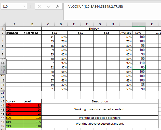
Also, I'd like to colour code the IF cells too but can't seem to make this work. Here's what I've got so far:

Thanks

Catherine

[#2]

Hello,

do you have a table with static values in cell A44 to A48? Do you want the formula to always look at these cells? Then you can use absolute references, with $ signs in front of the column letter and the row number, i.e. $A$44 instead of A44. Then, when the formula is copied down, it will still refer to $A$44.

Is there a reason you put the numbers into quotes, like "85" instead of just 85? That will return them as text and you can't easily use the values in calculations later on.

It is also better to use a lookup formula to look up the values instead of hard-coding them into the formula. That way, if your level definitions ever change, you only need to change the number in one place.  For example,  put the threshold values into A44 to A49 and in B44 to B49 put the result values. then you can use

=VLOOKUP(I3,$A$44:$B$49,2,TRUE)

With TRUE as the last parameter, Vlookup will use an approximate lookup which is perfect for lookups for numbers in a range from x to z.

[#3]

Hi,

Thank you so much for your help, using the  VLOOKUP that you suggested worked perfectly!

Can you / anyone else help with the conditional formatting that I'd like to use to colour code the cells in column J? I still can't get it to work.

thanks

Catherine

[#4]

Hi again,

On closer inspection the VLOOKUP hasn't worked - it isn't showing the correct results. J10 & J14 should read 90, J7, J8 & J15 should read 95. I'm really not familiar with this so I've probably done something silly! I've attached a screenshot

[#5]

Trouble is that the 37 % isn't in your block of answers for the vlookup and then will give the last value that fits e.g. after the 20% There will be masters here that can give better answers but I would make a long if statement or make a new table from 1 to 100 on another tab and use that one for the vlookup. The table on the current can stay there for reference but wil be not used by excel then .

regards,

Willie

[#6]

The longer if statement being '=IF($E$43<A44,B44,IF($E$43<A45,B45,IF($E$43<A46,B46,IF($E$43<A47,B47,IF($E$43<A48,B48,IF($E$43<A49,B49))))))'

Keep in mind I absolute adressed the $e$43. on that spot should be the cell you check .

Hope it helps a bit

For the coloring you can use the standard conditional formatting for one color. You just have to put them in right order since the will be examined in the list order you see when you open conditional rules.