IF Function help!

[JunSheng]

Hello, I am trying to add the IF function to a number of cells horizontally for a set of data vertically using autofill

To understand this better, ill use this function as an example: =IF(ISBLANK(B22), 0,1), and the cell im typing this on is A1.

So, if B22 is empty, itll display a "0". If i have data from B22 to B30, and i want the cells that display 0 or 1 from A1 to H1, I would fill in the function one by one. I tried autofilling cell A1 to H1 after typing the function in cell A1 but it shows =IF(ISBLANK(C22), 0,1) in cell B1 instead of =IF(ISBLANK(B23), 0,1), and so on. 

Sorry if my explanation is bad, i am still trying to get used to excel. Thank You!

[#2]

You may enter this formula in A1, copied across to H1:
=(INDEX($B22:$B30,COLUMN())<>"")*1

[#3 · Accepted solution]

@JunSheng 

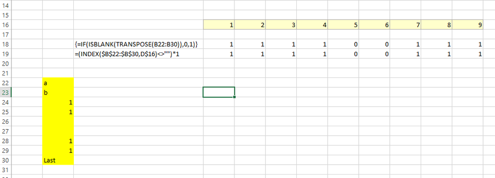
If you go with @Twifoo 's suggestion I'd recommend typing in the column references (see yellow cells) rather than relying on the COLUMN() formula, because if someone inserts a column A then you'll get the wrong results

Another option is to use the Transpose Function combined with entering it as an array (pressing Ctrl+Shift+Enter) to get the curly brackets.  But if you are new to Excel this will be confusing.

I've attached an example file

[#4]

@Wyn Hopkins 

I so wish the ridiculous idea of referencing by location had never been invented; it is pure junk!

Once one gets to meaningful problems most models require database tables or functions of time, i.e. lists and arrays.  A notation that encourages one to reference individual cell by location rather than business objects in their entirety fails to capture the intent of any solution.

In this case I would argue that

= TRANSPOSE( SIGN(list<>"") )

is far clearer than any filled formula.

p.s. … and, with dynamic arrays, the formula only requires one to use a single cell for the formula!

[#5]

@Wyn Hopkins 

Thank you so much!

[#6]

@Peter Bartholomew Thank you!

[#7]

@Twifoo Thank you!