- Home
- Microsoft 365
- Excel
- How can I insert a search box into a spreadsheet that searches comma separated values in cells?
How can I insert a search box into a spreadsheet that searches comma separated values in cells?
- Subscribe to RSS Feed
- Mark Discussion as New
- Mark Discussion as Read
- Pin this Discussion for Current User
- Bookmark
- Subscribe
- Printer Friendly Page
Jul 25 2019 05:48 PM - edited Aug 14 2019 12:20 AM
- Mark as New
- Bookmark
- Subscribe
- Mute
- Subscribe to RSS Feed
- Permalink
- Report Inappropriate Content
- Mark as New
- Bookmark
- Subscribe
- Mute
- Subscribe to RSS Feed
- Permalink
- Report Inappropriate Content
Jul 25 2019 06:26 PM
@Deleted
Hi
The function used to search for a keyword is called "Search"
If you type "Apple" as a keyword in Cell B1 and you want to search in the Range A5:A50 for the existence of this keyword,
You can type IsNumber(Search($B$1,A1)) >> and copy it all the way down >> it will return a TRUE if the keyword exists and a FALSE if the keyword does not exist
Using this concept with an advanced filter enables you to extract the record having the keyword.
If you have multiple keywords then, you need to include your function in an OR function and put the keywords in separate cells.
Should you wish a more customized answer then post an Excel spreadsheet with sample data.
Thanks
Nabil Mourad
- Mark as New
- Bookmark
- Subscribe
- Mute
- Subscribe to RSS Feed
- Permalink
- Report Inappropriate Content
Jul 26 2019 03:11 AM
@Deleted
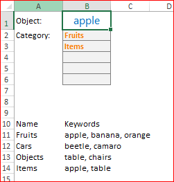
For such sample
you may use B1 to enter terms, in B2 add the formula
=IFERROR(INDEX($A$11:$A$14,AGGREGATE(15,6,1/ISNUMBER(SEARCH($B$1,$B$11:$B$14))*(ROW($B$11:$B$14)-ROW($B$10)),ROW()-ROW($B$1))),"")and drag it down.
Please see attached.
- Mark as New
- Bookmark
- Subscribe
- Mute
- Subscribe to RSS Feed
- Permalink
- Report Inappropriate Content
Jul 26 2019 07:54 AM - edited Aug 14 2019 12:21 AM
......
- Mark as New
- Bookmark
- Subscribe
- Mute
- Subscribe to RSS Feed
- Permalink
- Report Inappropriate Content
Jul 26 2019 09:53 AM
@Deleted ,
The workaround could be to wrap keywords by spaces and search for " apple ", not "apple", like
=IFERROR(
  INDEX($A$11:$A$14,
    AGGREGATE(15,6,
      1/ISNUMBER(SEARCH(" " & $B$1 & " "," " & SUBSTITUTE($B$11:$B$14,","," ")))*
        (ROW($B$11:$B$14)-ROW($B$10)),
      ROW()-ROW($B$1)
  )
  ),
"")
If there are spaces within your keywords you may use any other character instead of space. Please check attached.
- Mark as New
- Bookmark
- Subscribe
- Mute
- Subscribe to RSS Feed
- Permalink
- Report Inappropriate Content
Jul 31 2019 01:44 PM - edited Aug 14 2019 12:21 AM
......
- Mark as New
- Bookmark
- Subscribe
- Mute
- Subscribe to RSS Feed
- Permalink
- Report Inappropriate Content
Jul 31 2019 02:29 PM
@Deleted
Okay, I'll try.
Let start from wrapping - by SUBSTITUTE the comma on space and adding the leading space we are sure what each keyword in the string is starts and end with space, e.g we have " table chairs " instead of "table, chairs". Adding spaces to lookup value we ensure what SEARCH find only full keywords. Search of " tab " returns an error, only " tables " gives some result. Without that we find with correct result "tab" in "table, chairs".
ISNUMBER returns TRUE if SEARCH found the keyword and FALSE otherwise. In arithmetic operations TRUE and FALSE are equivalent to 1 and 0.
With AGGREGATE we find nth (last parameter, ROW()-ROW($B$1)) smallest (first parameter 15) value in the array ignoring all errors (second parameter 6).
Our array here 1/ISNUMBER(...) as before which returns an error (1/0) or 1 (1/1) depends on found keyword in records of the range $B$11:$B$14 or not; and multiplied on sequential number of row in this range. If keyword in first and fourth category record, resulting array will be like {1,error,error,4}. For the first cell AGGREGATE returns first smallest value (1), for the next cell second smallest value ignoring errors (4), and for the third cell an error will be returned since we have only two smallest values. Actually they are positions of records in Category keywords list.
INDEX takes these positions and returns Category names from $A$11:$A$14.
Finally IFERROR returns empty string if now keyword found.
To add current date you may add it to the value returned by INDEX like
=IFERROR(
  INDEX($A$11:$A$14,
    AGGREGATE(15,6,
      1/ISNUMBER(SEARCH(" " & $B$1 & " "," " & SUBSTITUTE($B$11:$B$14,","," ")))*
        (ROW($B$11:$B$14)-ROW($B$10)),
      ROW()-ROW($B$1)
  )
  ) & "-" & TEXT(TODAY(),"yyyymmdd"),
"")- Mark as New
- Bookmark
- Subscribe
- Mute
- Subscribe to RSS Feed
- Permalink
- Report Inappropriate Content
Jul 31 2019 02:31 PM
@Deleted
This new editor doesn't allow to attach the file, it's the same as previous time, only TEXT(...) is added to the formula.
