Help using index and match to find value based on 3 criteria

[calof1]

Hi,

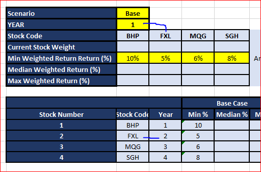
I have a large data set that involves three criteria, being year, scenario and product.

I am hoping to use a formula to find find and return the relevant answer from the data table. Attached is an example.

I have tried index and match, yet to find the right combination.

Can someone please assist.

Many thanks,

[#2]

@calof1 

Hey,

you could use the SUMPRODUCT formula instead:

Have a look at this video to understand how to use it: https://www.youtube.com/watch?v=lzjc_eEISe8

[#3 · Accepted solution]

@calof1 

The logic is bit unclear. You have 3 criteria - Scenario, Stock Code and Year. In source data you have no combination Stock Code=FXL and Year=1, however in answers you suggest 5% for Year=2. Why?

If ignore above formula could be

=IFERROR(
    INDEX($C$12:$S$15,
        MATCH(1,INDEX(($C$12:$C$15=C$4)*($D$12:$D$15=$C$3),0),0),
        MATCH(TRUE,ISNUMBER(SEARCH($C$2,$C$10:$S$10)),0)),
"N/A")

Couple of more comments. Your file is practically not downloadable, perhaps due to comma in name - not all system support it.

I'd recommend not to use Merging Cells. Potentially you will have lot of issues continue using merging. Alternative is - select sequential horizontal cells and apply Center Across Selection

[#4]

Hi@Sergei Baklan 

Thank you again for your help. Your solution works perfectly, and i appreciate your additional knowledge regarding merge cells. As a relatively new excel user i greatly appreciate all information and assistance.

Thanks again

[#5]

HIi@Sergei Baklan 

Thanks for your help. 

From the formula i notice it looks at case, scenario, year. I will columns for min, median, max and sd for each of these. Can this criteria be added to the formula?

Kind regards,

[#6]

@calof1 

To simplify the things you may define constants in Formulas->Name Manager as

when formula for the median is modified as

=IFERROR(INDEX($C$12:$T$15,
    MATCH(1,INDEX(($C$12:$C$15=C$4)*($D$12:$D$15=$C$3),0),0),
    MATCH(TRUE,ISNUMBER(SEARCH($C$2,$C$10:$T$10)),0)+ShiftMedian),
"N/A")

Sure you may use simply +0 or +1 or +2 or +3 in that part of formula.

[#7]

Hi Sergei@Sergei Baklan 

Thank you kindly again for your assistance. I am learning a lot, very much appreciated.

Kind regards,

[#8]

@calof1 , you are welcome