Help to find relevant data across multiple tabs of data. I think it is a index, match 3D formula

[calof1]

Hi Everyone,

I have a spreadsheet that has large number of tabs which are set up identically, there is just one tab for each product. Then lastly there is a summary tab. I want help with a formula to find and return the relevant data from each tab. I believe it is a combination of Index and match across the tabs.

Attached is an example.

Appreciate any help.

Kind regards,

[#2]

Which version of Excel are you using precisely? This is something you could do using PowerQuery (Get & Transform, New Query, From File, From Workbook)

[#3]

Hi Jan,

Thanks for the message.

I use Microsoft 2016 I believe. I have not used power query before however, but keen to learn.

Thanks

[#4]

@calof1 Here are the steps:

1. Save the file
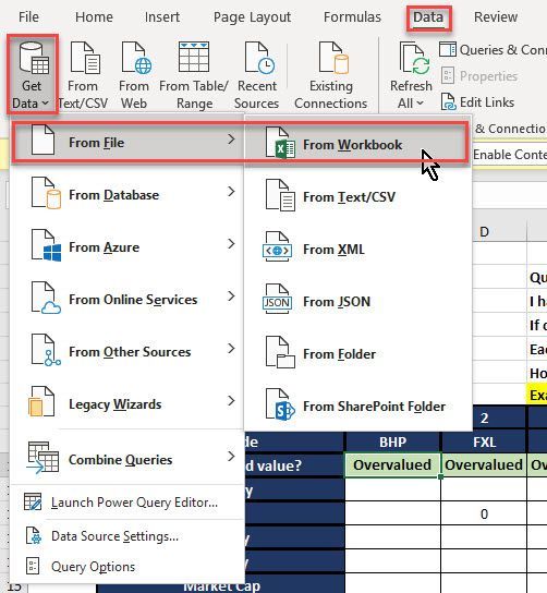
2. Click Data, Get Data (your button might be named "New QUery), From File, From Workbook:
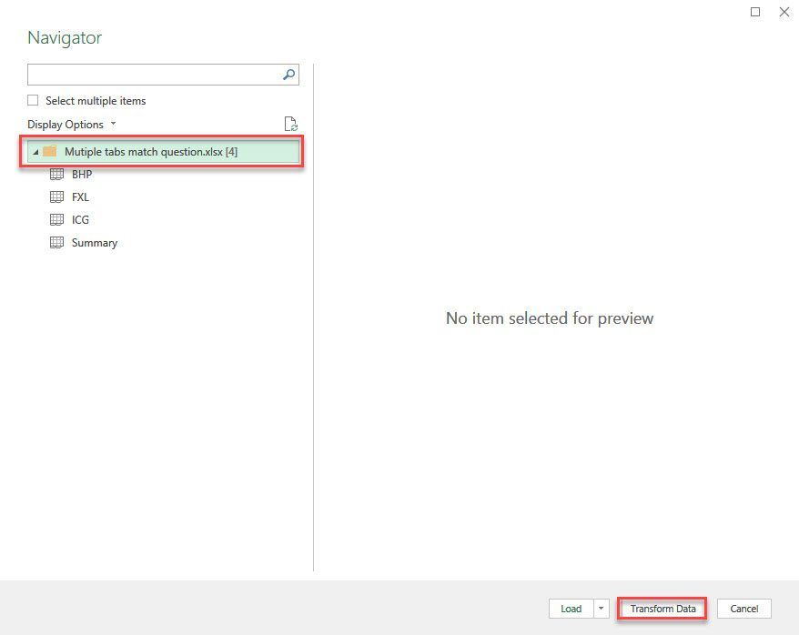
3. Click on the file name and then click Transform data:
   
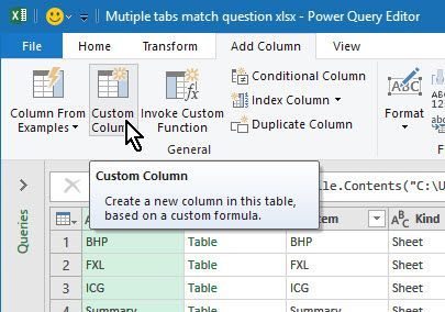
4. I assumed the tabs we wantto include all have three-letter names. Click the Add column tab, Custom Culomn button:
   
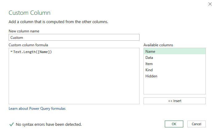
5. Use this formula to calculate the # of characters in the tab name:
   
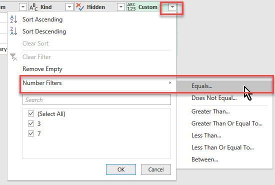
6. Click the filter button on the new column and select "Number filters", "Equals...":
   
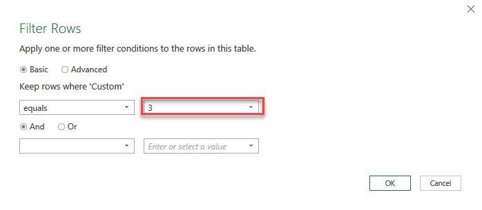
7. Set it to 3:
   
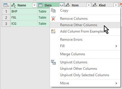
8. Select the first two columns by control-clicking their headers and right-click. Select "Remove other columns":
   
9. Click the expander icon next to Data:
   
10. Keep all columns selected and OK the dialog.
11. Delete all columns you do not need
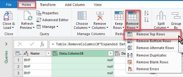
12. Remove the first 15 rows:
    
    
13. Click "Use first row as headers":
    
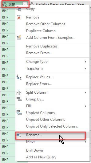
14. Rename first column back to "Name":
    
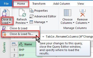
15. Click "Close and Load", Close and load to...:
    
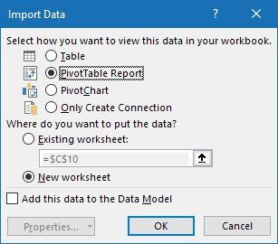
16. Choose these settings:
    
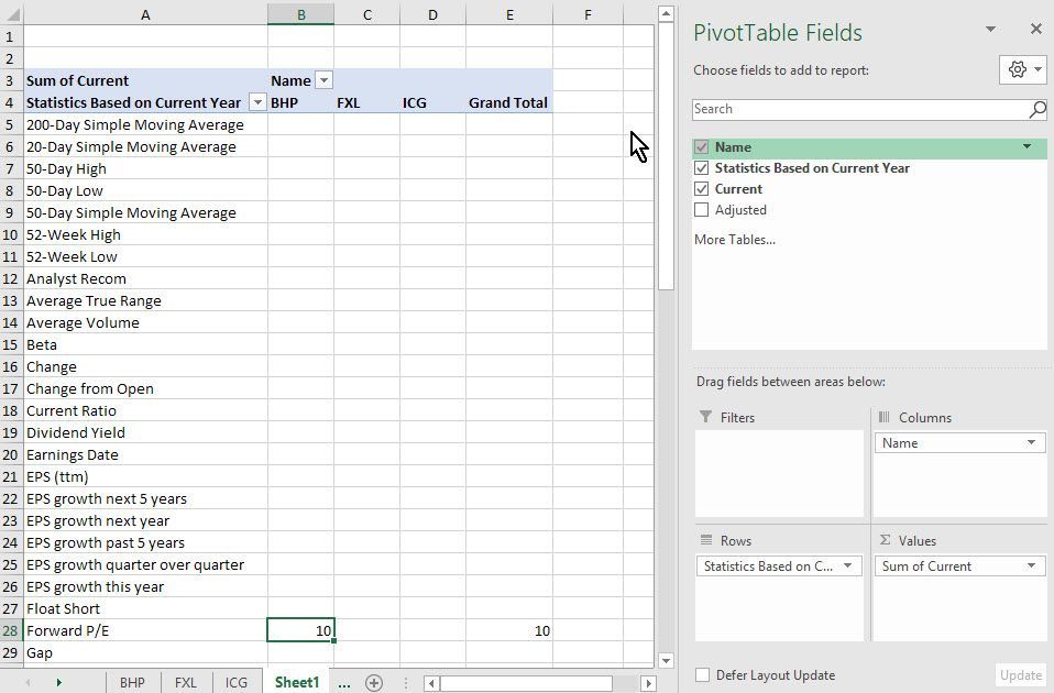
17. Now you're ready to create a pivot table which looks like your current report:
18. 

[#5]

Hi@Jan Karel Pieterse 

Thank you very much for the step by step instructions. I have been able to create a pivot table however it is slightly different to yours. For the "Statistics based on current Year" is this a named range created in the query? My attempt thus far is showing data from my first tabs of data, which i do not need to include.

I have attached what i am working on, the pivot table is located on row 125 down of the "Summary of Stocks" tab. Can you please see if you can tell what i need to amend in the query?

Thank you again for your support, much appreciated.

[#6]

Looks like you at least did not filter the calculated column containing the length of the worksheet names to 3 characters. Also you didn't remove the unneeded columns. The steps are there in my instructions :)