Help adding on to an iferror calculation

[debbienz]

Forgive my lack of Excel understanding, but I need help.

I have a client who wants to see the change in sales from one month to the next. Often, one month will be blank.

• The client wants when there is a new month of sales to show +100%.
• When the new month has no sales, and the prior month did, to show -100%.
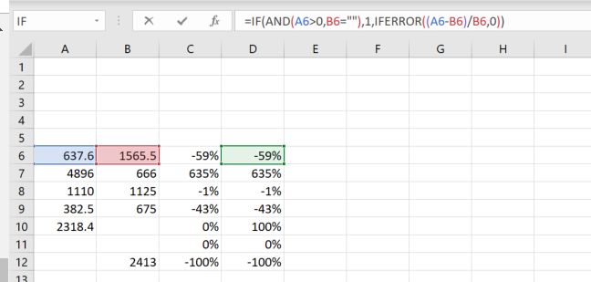
• The iferror statement works to show the -100%. However it returns a 0 for when sales are recorded, instead of the +100% I'll show it below 

(by the way is this the best way to do this?)

637.6	1565.5	-59%	=IFERROR((A6-B6)/B6,0)
4896	666	635%	=IFERROR((A7-B7)/B7,0)
1110	1125	-1%	=IFERROR((A8-B8)/B8,0)
382.5	675	-43%	=IFERROR((A9-B9)/B9,0)
2318.4		0%	=IFERROR((A10-B10)/B10,0)	client wants +100
		0%
	2413	-100%	=IFERROR((A12-B12)/B12,0)

[#2]

Kia ora @debbienz ,

try this in D6 and copy down:

=IF(AND(A6>0,B6=""),1,IFERROR((A6-B6)/B6,0))

[#3]

@debbienz 

Hi

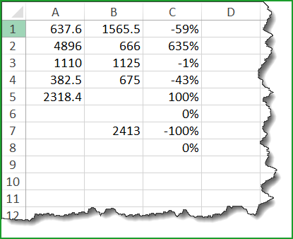
If I understand properly, here is a solution for you with a sample file

I used this formula in Cell C1

=IF(AND(A1<>"",B1=""),1,IF(AND(A1="",B1=""),0,(A1-B1)/B1))

there are 3 situation

1. both columns A & B have values
2. A has value, B doesn't
3. B has value , A doesn't

 Hope that helps

Nabil Mourad

[#4]

@Ingeborg Hawighorst 

THANK YOU!!!! THANK YOU!!!!! THANK YOU!!!!! 

Works a charm

[#5]

@nabilmourad 

Nabil 

THANK YOU!!!! THANK YOU!!!!! THANK YOU!!!!! 

Works a charm

[#6]

@Ingeborg Hawighorst Another question if you don't mind.

I've shared the link of the terrible excel sheet I've been given to fix up. The current excel sheet they have is over 100 column wide as you can see.. They are comparing three different criteria (current/ last income; current last no# cards presented and current/last commission paid. it's comparing one month to the same the prior year AND then adding on totals to the end.

So as you can see  It's currently un-workable!!!!!

I realise I'm not skilled enough to come up with a good solution for them to make this an easier workable spreadsheet.

Does anything stand out to you to change? If we separated years on different worksheet tabs, what would the formula you sent me be if instead ir was added onto a 3D cell reference?

Or can you think of a better solution?

Here's the dropbox link to the excel sheet https://www.dropbox.com/s/mdr6o746gp4amog/tech%20example.xlsx?dl=0 

[#7]

Hello @debbienz ,

The problem here is that the data is being entered into a report format, which makes it very, very hard to analyse and focus on specific areas of the data. A better way to handle this is to create a flat data entry table with the following columns:

- Activity type (i.e. Revenue, Card usage, Commission)

- Company name

- commission %

- Date

- value

This table will have a lot of rows, but just these four columns. With this flat table you can build a pivot table and calculate the differences. The pivot table can be made to look similar to your existing layout, or you can create different pivot tables to focus on different aspects of the data.

With pivot tables, the report can be filtered and show the insights that are relevant without scrolling dozens of pages.

This is too complex to answer in a single question, but the data can be converted with Power Query (Get & Transform) on the Data ribbon, and you may want to catch a tutorial on pivot tables to get you started.