- Home
- Microsoft 365
- Excel
- Re: HOW TO: "If cell contains specific text then return specific text"
HOW TO: "If cell contains specific text then return specific text"
- Subscribe to RSS Feed
- Mark Discussion as New
- Mark Discussion as Read
- Pin this Discussion for Current User
- Bookmark
- Subscribe
- Printer Friendly Page
May 12 2017
03:14 PM
- last edited on
Jul 25 2018
09:36 AM
by
TechCommunityAP
- Mark as New
- Bookmark
- Subscribe
- Mute
- Subscribe to RSS Feed
- Permalink
- Report Inappropriate Content
May 12 2017
03:14 PM
- last edited on
Jul 25 2018
09:36 AM
by
TechCommunityAP
I'm trying to extract a bunch of specific text combinations from cells and present it in a new cell.
This formula seems to work for two variables but I can't add any more variables too it.
=IFERROR(IF(SEARCH("*Sales*",B3,1),"Sales"),IF(SEARCH("*Arch*",B3,1),"Architecture"))
The text I would be searching for would be:
Sales,
Arch,
Land,
ALL,
Contracts,
Construction
and possibly a couple more.
Is there a way to do this?
- Labels:
-
Formulas & Functions
-
Requests
- Mark as New
- Bookmark
- Subscribe
- Mute
- Subscribe to RSS Feed
- Permalink
- Report Inappropriate Content
May 27 2019 11:10 AM
I am looking for a formula to do the following. I believe it is an "IF", but not sure. I basically want a formula to return results based on the following:
If the cell with the number is <=50, then multiply by 2
If the cell with the number is >50, but <=100, then multiply by 1.75
If the cell with the number is >100, but <=200, then multiply by 1.50
I am trying to combine in one formula so that I can copy it all the way down the spreadsheet. Any help would be greatly appreciated.
- Mark as New
- Bookmark
- Subscribe
- Mute
- Subscribe to RSS Feed
- Permalink
- Report Inappropriate Content
Aug 16 2019 03:40 AM
@Detlef Lewin Thank you so much - I spent so long looking for this - it works perfectly!
- Mark as New
- Bookmark
- Subscribe
- Mute
- Subscribe to RSS Feed
- Permalink
- Report Inappropriate Content
Aug 16 2019 04:13 AM
=A1*IF(A1>200,1,IF(A1>100,1.5,IF(A1>50,1.75,2)))
or
=A1*LOOKUP(A1,{0,50.000001,100.000001,200.000001},{2,1.75,1.5,1})- Mark as New
- Bookmark
- Subscribe
- Mute
- Subscribe to RSS Feed
- Permalink
- Report Inappropriate Content
Oct 28 2019 01:30 AM
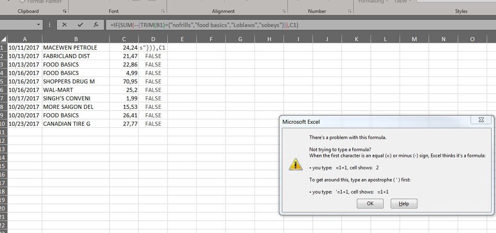
@Sergei Baklan this is exactly what I`m looking for but excel gives me an error - attached.
Could you please help?
- Mark as New
- Bookmark
- Subscribe
- Mute
- Subscribe to RSS Feed
- Permalink
- Report Inappropriate Content
Dec 30 2019 10:40 AM
@Detlef Lewin This works perfectly in most situations and is super simple, so I want to thank you for providing this! I haven't seen this solution offered anywhere else! The only problem I sometimes run into is that this isn't an exact match, so if I have a list of text that has some of the same terms or letter combinations, it sometimes returns the wrong thing. Is there a way to make this exact match only?
- Mark as New
- Bookmark
- Subscribe
- Mute
- Subscribe to RSS Feed
- Permalink
- Report Inappropriate Content
Dec 30 2019 11:00 AM
Could you please attache the file instead of screenshort.
- Mark as New
- Bookmark
- Subscribe
- Mute
- Subscribe to RSS Feed
- Permalink
- Report Inappropriate Content
Feb 11 2020 03:06 AM
@Sergei Baklan I really like your solution with nested formatting, though I was wondering if there is a way to efficiently do a few hundred words?
There must be a better option than typing in all the words
- Mark as New
- Bookmark
- Subscribe
- Mute
- Subscribe to RSS Feed
- Permalink
- Report Inappropriate Content
Feb 11 2020 07:48 AM
I gave nested IF only to illustrate that is workable. Formula which @Detlef Lewin suggested shall work perfectly, especially on big ranges.
- Mark as New
- Bookmark
- Subscribe
- Mute
- Subscribe to RSS Feed
- Permalink
- Report Inappropriate Content
Apr 18 2020 11:02 PM
@Reuben I am working on a spreadsheet that contains macros. In column A, users input an 'X' to make that row active which then gets copied for an email. If the row does not contain an 'X', the row is hidden and not copied for an email.
So what I am trying to accomplish:
IF a range of cells don't contain an 'X', THEN display "general text message".
If none of the cells from A2 through A10 contain an 'X', then I want a message to be displayed in B1. However, if any of the cells from A2 though A10 contain an 'X', then B2 should not display a message.
If there is a way to accomplish this, is it possible to have the formula automatically adjust to a new range of cells, ie. if I were to add a row between A2 and A10.
- Mark as New
- Bookmark
- Subscribe
- Mute
- Subscribe to RSS Feed
- Permalink
- Report Inappropriate Content
May 15 2020 11:39 PM
I have a problemm where I need to filter out the state and district name from the address column and place the same in the adjoining column
State llist can be arranged as a range. But what would be the formula to use and how will it be used to math the address column
- Mark as New
- Bookmark
- Subscribe
- Mute
- Subscribe to RSS Feed
- Permalink
- Report Inappropriate Content
May 25 2020 03:06 PM
Hi was googling for a solution to the subject of above thread and found and used your solution,
[Key words in column F, returned text in column G, text to check in A1.
=LOOKUP(PI(),1/COUNTIF(A1,"*"&$F$1:$F$6&"*"),$G$1:$G$6) ]with 1 problem; the keyword found doesn't display.
using Excel 2010
would appreciate any help
thanks!
- Mark as New
- Bookmark
- Subscribe
- Mute
- Subscribe to RSS Feed
- Permalink
- Report Inappropriate Content
May 27 2020 08:18 AM
- Mark as New
- Bookmark
- Subscribe
- Mute
- Subscribe to RSS Feed
- Permalink
- Report Inappropriate Content
Nov 04 2020 07:35 AM
- Mark as New
- Bookmark
- Subscribe
- Mute
- Subscribe to RSS Feed
- Permalink
- Report Inappropriate Content
Nov 04 2020 10:52 AM
Not sure what exactly you'd like to do, perhaps something like
= Table.SelectRows(
  #"Table To Filter" ,
  each List.Contains(
         #"Table With Filter"[ColumnWithValues],
         [ColumnOnWhichWeFilterSourceTable]
        )
)
- Mark as New
- Bookmark
- Subscribe
- Mute
- Subscribe to RSS Feed
- Permalink
- Report Inappropriate Content
Nov 04 2020 11:58 AM
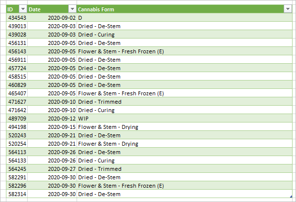
@Sergei Baklan we have a data cleanliness issue, whereby a freeform field contains key information about each entry. Inside the freeform field are keywords which we want to pull out into a new column. The =LOOKUP(PI(),1/COUNIF(TargetCell,"*"&KeywordRange&"*"),KeywordRange) Formula works well in an Excel sheet, however our dataset is much larger and we will need to handle it in PQ or some other tool. Essentially we want perform the same operation as the above function but within PQ.
I have attached a sample of the dataset, with tables showing the raw data and target keywords (INPUTS) as well as a sample output of cleaned data (OUTPUT). I achieved the example output by using a fuzzy match in PQ, but that is not necessarily a perfect resolution. Perhaps it works.
Cheers,
- Mark as New
- Bookmark
- Subscribe
- Mute
- Subscribe to RSS Feed
- Permalink
- Report Inappropriate Content
Nov 04 2020 01:06 PM
I' not sure how the table with keywords works. For example, keyword a is met in every word for several times. Thus simply try to reproduce what LOOKUP() do. Second part of your query, instead of fuzzy merging, is
    #"Lowercased Text" = Table.TransformColumns(
        #"Removed Columns",
        {{"Description", Text.Lower, type text}}
    ),
    KeywordsTable = CannaFormKeywords,
    #"Add Cannabis Form" = Table.AddColumn(
        #"Lowercased Text",
        "Cannabis Form",
        each
            let
                txt = [Description],
                lst = KeywordsTable[Keyword],
                out = KeywordsTable[Cannabis Form],
                transformed = List.Transform(
                    lst,
                    each
                        if Text.Contains(txt, _)
                        then out{List.PositionOf(lst,_)}
                        else null
                ),
            cleaned =
                List.Last(
                    List.RemoveNulls(
                        transformed
                    )
                )
            in
                cleaned),
    #"Remove source texts" = Table.SelectColumns(
        #"Add Cannabis Form",
        {"ID", "Date", "Cannabis Form"}
    )
in
    #"Remove source texts"
(see duplicated query).
Result looks the same as with fuzzy match
- Mark as New
- Bookmark
- Subscribe
- Mute
- Subscribe to RSS Feed
- Permalink
- Report Inappropriate Content
Dec 10 2020 05:29 PM
=IFERROR(INDEX($G$1:$G$6,AGGREGATE(15,3,SEARCH($G$1:$G$6,A1)*ROW($G$1:$G$6),1),1), "No Match")

* AGGREGATE can ignore error- Mark as New
- Bookmark
- Subscribe
- Mute
- Subscribe to RSS Feed
- Permalink
- Report Inappropriate Content
Dec 10 2020 11:37 PM
Sorry, I didn't catch what's that about. If about recent post, I'd prefer formula which @DMColleran used before
=LOOKUP(PI(),1/COUNTIF(TargetCell,"*"&KeywordRange&"*"),CannabisRange)it works better than SEARCH() within AGGREGATE().
As for the concrete formula, it won't work for the sample from previous post, shall be adjusted.
- Mark as New
- Bookmark
- Subscribe
- Mute
- Subscribe to RSS Feed
- Permalink
- Report Inappropriate Content
May 05 2021 09:36 PM
I agree and your value add help me no end. Thanks and keep up the great dialogue.
- « Previous
-
- 1
- 2
- Next »

