Find matching values in column cells and the sum of of the cells in the rows of each matching cell

[Bill McDavid]

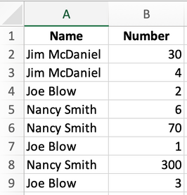
I am at a complete loss on how to do this and I am hoping for some help. Probably easiest to demonstrate with two images below with a small set of hypothetical data. In the first image, you can see column A has duplicated values. The formula I hope to build is one that will find all values in column A that match and then add up all the values in Column B that correspond to the matching cells in Column A. For example, there are two cells in Column A that have a value of Jim McDaniel and values in Column B are 30 and 4 (sum of 34 for Jim McDaniel). 

On a summary worksheet, I would like the results of the first worksheet to be displayed as per the example below. I'd like one row for each of the matching values from Column A from the first worksheet and then Column B would show the sum of the values from the corresponding values from Column B in the first worksheet. 

Any and all help is MUCH APPRECIATED!!

[#2 · Accepted solution]

Hi Bill,

The easiest way to do this is by using the PivotTable as the below screenshot:

To learn more about PivotTables, please check out this link and this.

Hope that helps

[#3]

This is SO helpful! Thank you! Here is a followup question. Do you know if there is a way to automatically delete from the first sheet the rows that have an aggregate value from Column B in the summary that have a value below a certain number? For example, if the threshold is "300" would it be possible to automatically delete the source data for Jim and Joe because their aggregated column B data is less than 300. I hope that makes sense. 

---

@Haytham Amairah wrote:

Hi Bill,

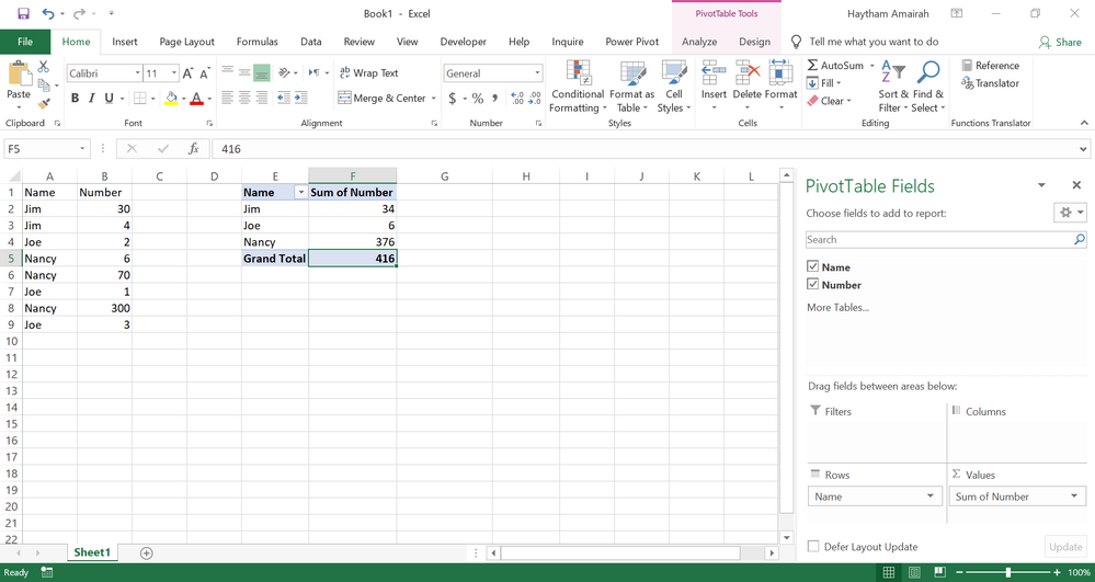
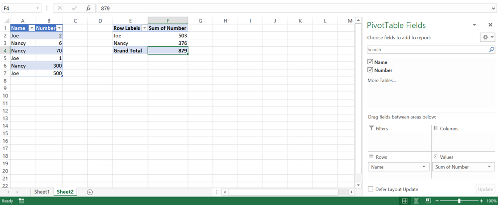
The easiest way to do this is by using the PivotTable as the below screenshot:

To learn more about PivotTables, please check out this link and this.

Hope that helps

---

[#4]

Hi Bill,

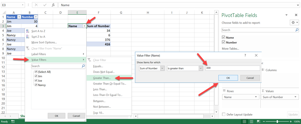
You can easily filter out the aggregations that don't meet certain criteria as the below screenshot:

Regards,

Haytham

[#5]

That is also helpful but I would ideally like to delete the source data. This is because in the end I need to go back to the source data and export 1 complete record (all fields from the source data) from each record shown on the filtered summary. Ideas?

[#6]

You can't delete the records in the source table that its aggregation is less than a certain threshold unless you use a Macro/VBA solution which it could be difficult!

But I have a fairly good and easy workaround for this case.

Before you create the PivotTable, please create another column in the source table that contains this formula:

=IF(SUMIF($A$2:$A$9,A2,$B$2:$B$9)>300,TRUE,FALSE)

 

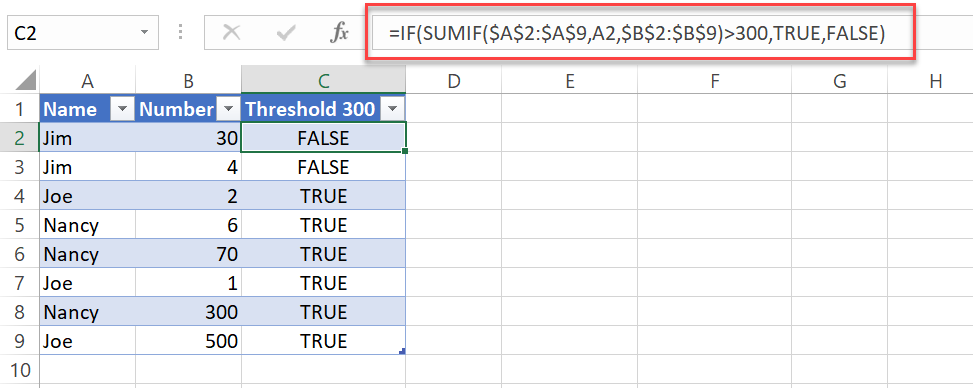
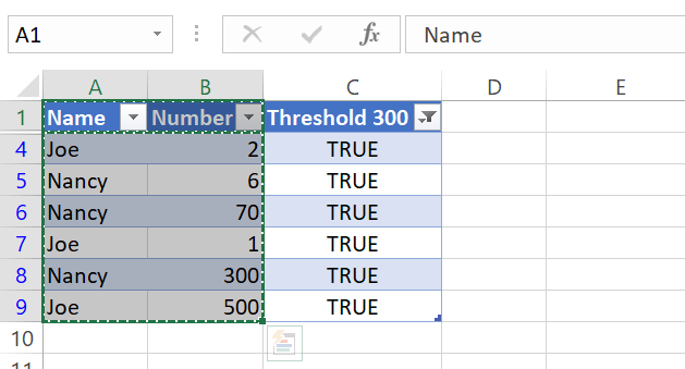
Then filter out the FALSEs and copy the filtered table into a new worksheet as below:

After that, create a new PivotTable from the new source table as below:

Regards

[#7]

You are a Godsend! Thank you!!

[#8]

@Haytham Amairah I am attempting to do something very similar but I am trying to match multiple columns/rows of data and bring back a sum.  Example below:  if A2-E2 match exactly A3-E3 then total the sum of those matching rows, which should come back as zero (8.2-8.2 or F2+F3).  I put this all in a pivot but need the zeros to not show.  I only need the unique row's sum, and the comment needs to show for each one.  I appreciate any ideas.  I have tried a calculated field in a pivot but it wont pull the comments. 

Clock	Last	First	Event	Date	Sum	Comment
358	Smith	Joe	no show	2/10/2021	8.2	Test
358	Smith	Joe	no show	2/10/2021	-8.2	Test
358	Smith	Joe	no report	2/11/2021	8.2	Test
456	Smith	Ted	no show	02/01/2021	8.2	Test
456	Smith	Ted	no report	02/16/2021	-8.2	Test
456	Smith	Ted	no report	02/16/2021	8.2	Test
456	Smith	Ted	FMLA	02/15/2021	8	Test