Excel Multistep lookup function INDEX MATCH?

[CodeRed2004]

I need a formula that looks up a value based upon several other values. I'm pretty sure that it needs to be a custom macro formula or a index/match formula, but I'm not certain how to set it up.

Lookup value in a separate sheet by column # or header by PO>UPC>Appx referenced QTY

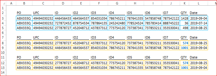
The top table (book 1) is where I'm pulling the data from. The bottom (book 2) is the table where I need to make the formulas to fill in the ID/Date information.

PO	UPC	ID	ID2	ID3	ID4	ID5	ID6	ID7	QTY	Date
ABX333Q	49494030232	446456433	464564537	854031034	786745211	787641335	547858748	787542122	1428	9/4/2019
ABX333Q	49494030232	727872452	878754534	787864135	245242480	778524524	785783414	888745222	36	7/14/2019
ABX333Q	49494030232	277878727	452048712	437837312	773754120	737387341	737853211	353530041	498	8/25/2019
PO	UPC	ID	ID2	ID3	ID4	ID5	ID6	ID7	QTY	Date
ABX333Q	49494030232								574

[#2]

Hello @CodeRed2004 ,

can you explain what the expected result would be in the lower table? The top table has three rows with the same PO and UPC.  What do you want to see in the lower table? And how does the number 574 get into the Qty column?

[#3]

@Ingeborg Hawighorst 

Each table comes from two different systems. The goal is to match them up. All the data in the bottom table is already provided. I'm trying to fill in the blanks with data from the top table. VLOOKUP does not work because it returns the first result. I need to the result that most closely matches the QTY in the bottom table. In this example the right answer would be the third row as the difference in QTY is the smallest. I would want that rows date and ID#s. Thanks for your help!

[#4]

@CodeRed2004 

What version of Excel are you using?

 I filtered the Quantity field by PQ and UPC

= ABS( FILTER(Table1[QTY],  (Table1[PO]=PO)*(Table1[UPC]=UPC ) ) - QTY )

and calculated the absolute difference between it and the target value QTY.

Then I sorted the ID and Date by these deviations 

= @SORTBY( ID.filtered, QTY.filtered )

and returned the value corresponding to the lowest deviation.

I haven't posted to workbook because the chance that you will be able to use it is remote.

[#5]

I'm using the Office 365 version.

[#6]

@CodeRed2004 

Since you are using Office 365, you will sooner or later get the FILTER and SORT functions I have used so I have attached a workbook.  At the moment, I believe they are being rolled out to 'monthly' update users.

The solution is highly non-standard so you might well be advised to see what @Ingeborg Hawighorst comes up with.

[#7]

@CodeRed2004 

In more traditional way for such sample

formulas could be like

=IFERROR(INDEX($D$3:$L$5,MATCH(1, INDEX( ($B8=$B$3:$B$5)*($C8=$C$3:$C$5)*(MIN(ABS($K$3:$K$5-$K8))=ABS($K$3:$K$5-$K8)),0),0),MATCH(D$7,$D$2:$L$2,0)),"no such")

or

=INDEX($D$3:$L$5,AGGREGATE(15,6,1/($B12=$B$3:$B$5)/($C12=$C$3:$C$5)/(MIN(ABS($K$3:$K$5-$K12))=ABS($K$3:$K$5-$K12))*(ROW($B$3:$B$5)-ROW($B$2)),1),MATCH(D$11,$D$2:$L$2,0))

[#8]

In the first formula I changed the targets to my actual targets which are in the main table and within another sheet. I checked and made sure they were right several times, but not avail. It just errored. Any ideas?

[#9]

@CodeRed2004 

It's hard to say without seeing the formula. Perhaps you may attache sample file which is structured as your actual one, but without sensitive data.