Excel Mac Pivot Charts - Can you switch rows and columns without changing the pivot table?

[Colm Ryan]

Hi, 

I love the new Pivot Chart feature on Excel 2016 for Mac. However sometimes I would like to Switch Rows and Columns on the chart without affecting the pivot table.

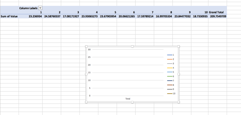
For instance, in a pivot table where amounts are organised on a horizontal timeline, if I try to do a line chart, I cannot see the timeline I would expect. I get something like this:

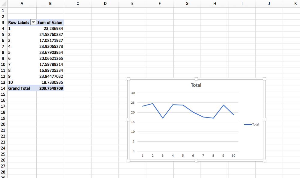
If I Switch Row and Column, I get this: 

This is the view I am looking for, however the pivot table is now showing a vertical timeline and not a horizontal timeline. This is not ideal, as I normally work with timelines in horizontal buckets.

Do you have any ideas as to how this can be rectified - ie a line chart from the second screenshot from a pivot table in the first screenshot?

Thanks,

Colm Ryan

[#2]

I'm having the same issue. Very annoying.

If your pivot table has time across columns, (ex: Jan, Feb, Mar - most common in finance) the pivot chart automatically uses that data for the y axis (instead of x).

How can this be switched?

[#3]

Hi Tom,

Pivot Chart is always has the same layout as connected Pivot Table. You may create and hide another Pivot Table to which your Pivot Chart will be connected; or create Power Chart only from data model with Power View (for Windows, not sure how it is on Mac)