Conditional formatting to highlight cell with higher than the average of the row.

[ESKARDA]

I have 52 weeks of shipping volume numbers sorted in 52 columns. The 53rd column is the average of the 52 weeks. Currently, I able to set a conditional format to high lite all cells in a particular row that are greater than the average in column 53. Can anyone tell me how to copy this format to the rest of the rows since they each have different averages. I dont want to set the same conditional format on over 1000 different shipping lanes. 

Edit: To simplify, each row is a different shipping lane. I want to highlight the weeks that exceed the lane's AVG cell as shown below. Is there a way to apply this format to the rest of the data without doing each individual shipping lane?

Volume: Week 45	Volume: Week 46	Volume: Week 47	Volume: Week 48	Volume: Week 49	Volume: Week 50	Volume: Week 51	Volume: Week 52	AVG
3	6	11	12	27	21	22	10	4
0	0	4	12	7	6	0	0	1
15	21	23	10	24	30	2	12	12

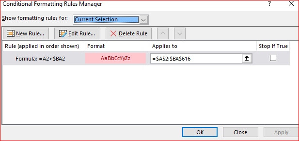
[#2 · Accepted solution]

@ESKARDA 

Use the rule with formula as

and apply it to your entire range. Only one rule. Just be careful with absolute and relative references.

Please check attached.

[#3]

@Sergei Baklan Ok so now I need to average those cells that are now highlighted. What is the best way to do that? I tried using the AVERAGIF formula but it is returning an error.

[#4]

@ESKARDA , I added formula into the next column

=AVERAGEIF($A2:$AZ2,">="&$BA2)

Please check attached 

[#5]

Your are my new favorite person!@Sergei Baklan