Conditional formatting cells by percentages

[Joshua Armstrong]

I am using office 2016. 

I have a document that I update daily. I am trying to have the top cell format red if there is a 20% discrepancy between the numbers. 

I add a new line every day, and copy/paste the numbers in (the blue numbers are the results of a formula)

I want to just add my line, put in the numbers and have it check the field below with the percentage and highlight if it's higher or lower than normal. 

[#2]

write this formula to Conditonal Formating->New Rule-->Use a formula to determine which cells to format

=ABS/($B2-$H2)/$B2)>0,2

and below line to Applies to:

=$A$1:$M$1

if you want to have the same rule applied in more rows change the row number in the last formula.ç

[#3]

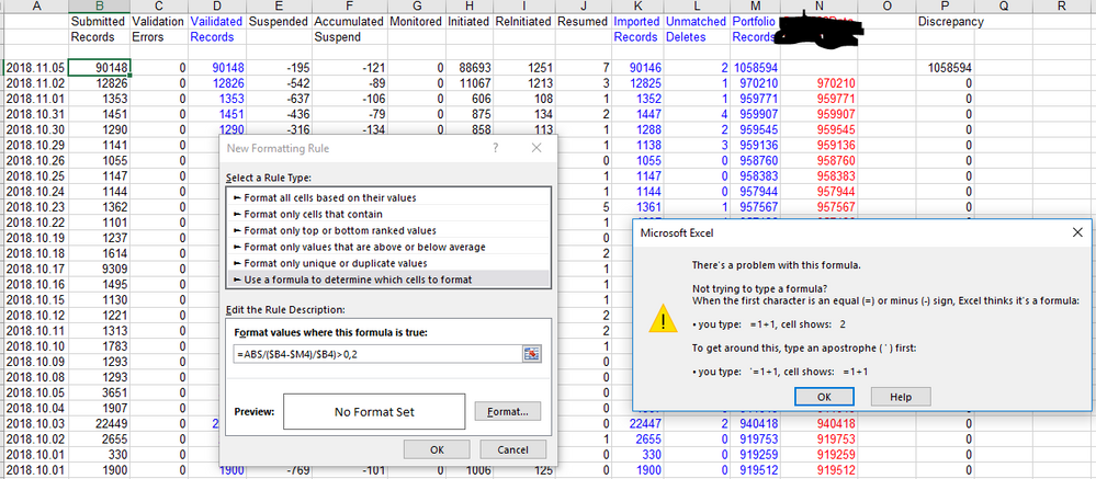
Got this error listed. I changed the corresponding cells accordingly. 

[#4]

Sorry there was a syntax error. It should have been

=ABS(($B2-$H2)/$B2)>0,2

[#5]

Thanks. Can you explain how the formula works so i can see how the calculation is processed? 

I'm still getting the same error code. 

If it helps to clarify, with the last screenshot I loaded. I wanted the value of B4 and B5 compared, and if B4 is more or less than 20% of B5, it would highlight. 

[#6]

First thing youı have to check is 0,2. Try changing it to 0.2

How formula works. This formula calculates the difference between $B2 and $H2 and divides the result with $B2 to find percentage and incase this value is negative ABS will convert it to a positive number. The trick here is "$" sign before column name and no signt before row number. This will cause excel to apply same formula to all the cell the formatting is applied with column names to be same in every row but take the row number from the actual row where the condition is checked. so basically the formula updates itself to =ABS(($B3-$H3)/$B3)>0.2; =ABS(($B4-$H4)/$B4)>0.2 and so on.