Conditional format based on formula results - Marlett font

[Tonya Troxtell]

Good Morning

I am using the following formula and would like to format the results based on the results of the formula.

=IF(C2<'2-1'!B2,"u",IF(C2>'2-1'!B2,"t","v"))

When shown in Marlett font, the "u", "t", and "v" show in arrows and I need to format based on the result of the arrow.  The goal is for the arrow cell to show a certain color.

[#2]

Hi Tonya Troxtell, you don't need to base on the result of the arrow.  You just need three conditional formatting rule on the arrow cells to base on your formula

1. for u
   

   =$C2<'2-1'!$B2

2. for t

   =$C2>'2-1'!$B2

3. for v

   =$C2='2-1'!$B2

[#3]

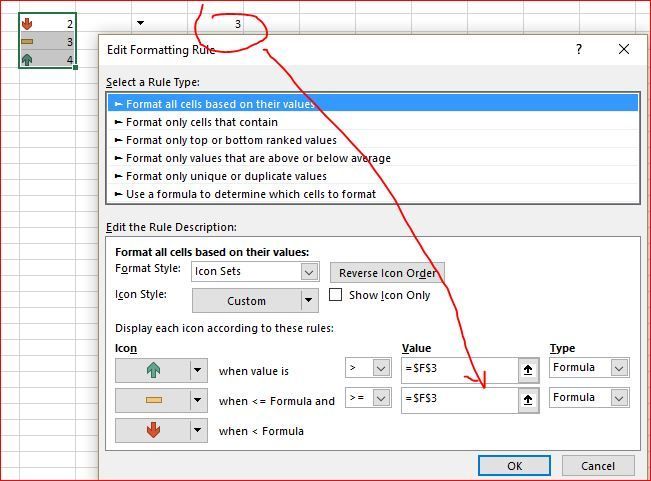
Alternatively you may use built-in into conditional formatting arrows icons set using formula for rules (and show icons only if desired)

[#4]

Will this formula work for the entire column or just the cell?

[#5]

Thanks! I did not know that was a feature.

[#6]

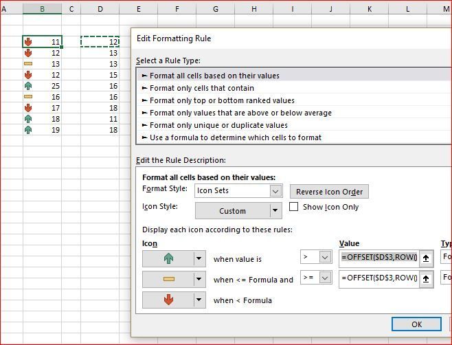
It works but with some tricks if you'd like to compare column-to-column. Icons sets works directly only with absolute reference, the workaround is to use OFFSET like

=OFFSET($D$3,ROW()-ROW($D$3),0)

for that data

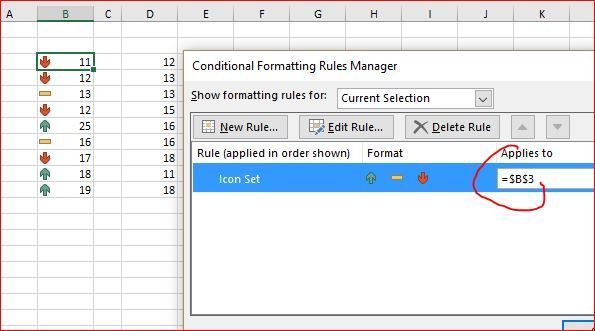
apply it only to first cell

and when Format Painter on entire column.