Conditional Formatting

[Squrt17]

I have a spreadsheet that has various certification dates in it.  Some expire in 3 years from the date entered, and some in 5 years.  I do NOT have any idea how to set up the conditional formatting so I can have the separate cells color coded depending on how far out they are from the original date entered.  I would like to have orange when they are 60-30 days out from expiration, and red when they are 29 and less.  I have a total of 4 different tests for about 100 people.  

[#2]

@Squrt17 , how the expiration is defined - do you have expiration date, or column where number  of years to expiration is defined (3 or 5) or what?

[#3]

@Sergei Baklan , currently there is nothing defined, but I can certainly do that if necessary.  The only thing in the columns are the dates the individuals took the certification test.  I just know when they expire...

[#4]

@Squrt17 

You need to share with Excel that your knowledge.

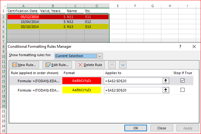
For sample date like this

you may apply two conditional formatting rules with formulas

for the red

=(TODAY()-EDATE($A2,$B2*12)<=29)*($A2>1)

yellow:

=(TODAY()-EDATE($A2,$B2*12)<=60)

If another range, instead of A2 it shall be top left cell of your range (excluding headers), B2 is in the same row years expiration column and be careful with absolute and relative references.