- Home
- Microsoft 365
- Excel
- Re: Conditional Formatting using multiple conditions
Conditional Formatting using multiple conditions
- Subscribe to RSS Feed
- Mark Discussion as New
- Mark Discussion as Read
- Pin this Discussion for Current User
- Bookmark
- Subscribe
- Printer Friendly Page
- Mark as New
- Bookmark
- Subscribe
- Mute
- Subscribe to RSS Feed
- Permalink
- Report Inappropriate Content
Jul 02 2019 09:14 AM
Hello
I was wondering if someone could help me.
I work in training within law enforcement and have made a spreadsheet to help me keep track of what hours the officers work each year to stay proficient. The hours are broken down into modules (A1.1, A1.2, A2.1 etc)
Every four weeks a team attends training and each day a lesson will be covered which will contain a number of hours of each type of module.
The spreadsheet has a list of the lessons and when an officer attends the lesson he will be marked as “attended”, this will then credit the officer with the appropriate amount of hours for each module contained within that lesson.
For example, Lesson A contains 1 hour module A1.1, 2 hours module A1.2 and 1 hour A2.1.
This will then add these hours to his scoresheet, by the end of the year the officer must have hit a certain number of hours on each module to stay proficient.
Each training cycle I also have an officer benchmark, which says that if the officer has hit every available lesson that has been provided he will to date have accrued this many hours.
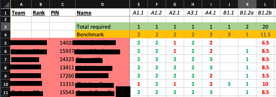
As the spreadsheet currently stands, if the officer has hit the "benchmark" hours then his number for that particular module then the number will turn green. If the Officer has not attended the amount of lessons that have been provided then the number will turn red.
However for some of the modules, the officer only has to accrue 1 hour for the year but the number of times that it will be hit in lessons will be more than that (see I5).
What i'd like to be able to do is this....
If the number is higher than the "Total Required" then turn the text green.
If the number is equal to the "Benchmark" but less than the "Total Required" then turn the text amber.
If the number is less than both the "Benchmark" and "Total Required" then turn the text red.
I'm not great with Excel and hope someone can help me with this. I'm sure it's probably a simple answer but any help would be appreciated.
Many thanks
Rob
- Mark as New
- Bookmark
- Subscribe
- Mute
- Subscribe to RSS Feed
- Permalink
- Report Inappropriate Content
Jul 02 2019 02:57 PM
SolutionYou need three conditional formatting rules, one for each color. Select your entire range (e.g. E5:L11 as on picture) and add new rule using the formula. For green it'll be
=E5>E$3
for amber
=(E5=E$4)*(E5<E$3)
and for the red
=(E5<E$4)*(E5<E$3)
Be careful with absolute and relative references.
- Mark as New
- Bookmark
- Subscribe
- Mute
- Subscribe to RSS Feed
- Permalink
- Report Inappropriate Content
Jul 02 2019 09:42 PM
- Mark as New
- Bookmark
- Subscribe
- Mute
- Subscribe to RSS Feed
- Permalink
- Report Inappropriate Content
Jul 03 2019 03:18 AM
@d32bus , you are welcome
Accepted Solutions
- Mark as New
- Bookmark
- Subscribe
- Mute
- Subscribe to RSS Feed
- Permalink
- Report Inappropriate Content
Jul 02 2019 02:57 PM
SolutionYou need three conditional formatting rules, one for each color. Select your entire range (e.g. E5:L11 as on picture) and add new rule using the formula. For green it'll be
=E5>E$3
for amber
=(E5=E$4)*(E5<E$3)
and for the red
=(E5<E$4)*(E5<E$3)
Be careful with absolute and relative references.