Conditional Formatting Formulas

[Briana_Valeriano]

In column A, I have 10 numbers. I want column B to have conditional formatting where if I enter a number that is higher than 70% of the value in column A, it will turn green. If it’s 70% or lower it will turn red.

[#2]

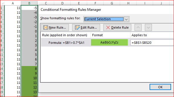
You may apply to column B conditional formatting rule for the green with formula 

=$B1>0.7*$A1

assuming your range starts from first row. Similar for the red rule.

[#3]

This works when I do it for just the first row but How do I apply that formula to all of column B. And not individually typing a formula for each cell in B

[#4]

It works for your entire range

Please see attached