Color-scale formatting dependent on each individual row in pivot table every three rows

[adisera]

Hi there,

      I have several problems I am running into- two questions in this discussion. The first one revolves around a pivot table I have which shows each individual item in our inventory, its description, and the three key data points for each (picture included below):

As you can see above I have a conditional format rule for a color scale that I wish to use to format the Supplier Network DOH key figure spanning across the six dates for each individual item like so:

However, I want to find a way to automate this process so I don't have to go through each individual row and use format painter with the 1000+ rows that I have to format. Important note to make as well as that whether I filter the pivot table to just Supplier Inventory DOH, or have all three key figures present, the conditional formatting cannot just be dragged and dropped as a blanket across all of the data- as each unique row of Supplier Inventory DOH (every three rows or so with the three figures present) only needs to be formatted-none of the other rows do. I found a similar related discussions referencing this article: https://stackoverflow.com/questions/51991016/excel-conditional-colour-scale-for-multiple-rows, and I tired inputting this code:

Option ExplicitSub ApplyConditionalFormatting()
    Dim ws As Worksheet: Set ws = ThisWorkbook.Sheets("Sheet1") ' change to your sheet here
    Dim rw As Long
    Dim rng As Range

    For rw = 3 To 8 ' change to your respective rows
        With ws
            Set rng = .Range(.Cells(rw, "E"), .Cells(rw, "K")) ' change to your respective columns

            With rng
                .FormatConditions.AddColorScale ColorScaleType:=3
                .FormatConditions(.FormatConditions.Count).SetFirstPriority  ' now its index is 1, in case there already was cond formatting applied
            End With

            With rng.FormatConditions(1)
                With .ColorScaleCriteria(1)
                    .Type = xlConditionValueNumber
                    .Value = 0
                    .FormatColor.Color = 7039480
                End With

                With .ColorScaleCriteria(2)
                    .Type = xlConditionValueFormula
                    .Value = "='" & ws.Name & "'!$D$" & rw & "*3" ' References column D, change as needed
                    .FormatColor.Color = 8711167
                End With

                With .ColorScaleCriteria(3)
                    .Type = xlConditionValueFormula
                    .Value = "='" & ws.Name & "'!$D$" & rw & "*5" ' References column D, change as needed
                    .FormatColor.Color = 8109667
                End With
            End With
        End With
    Next rwEnd Sub

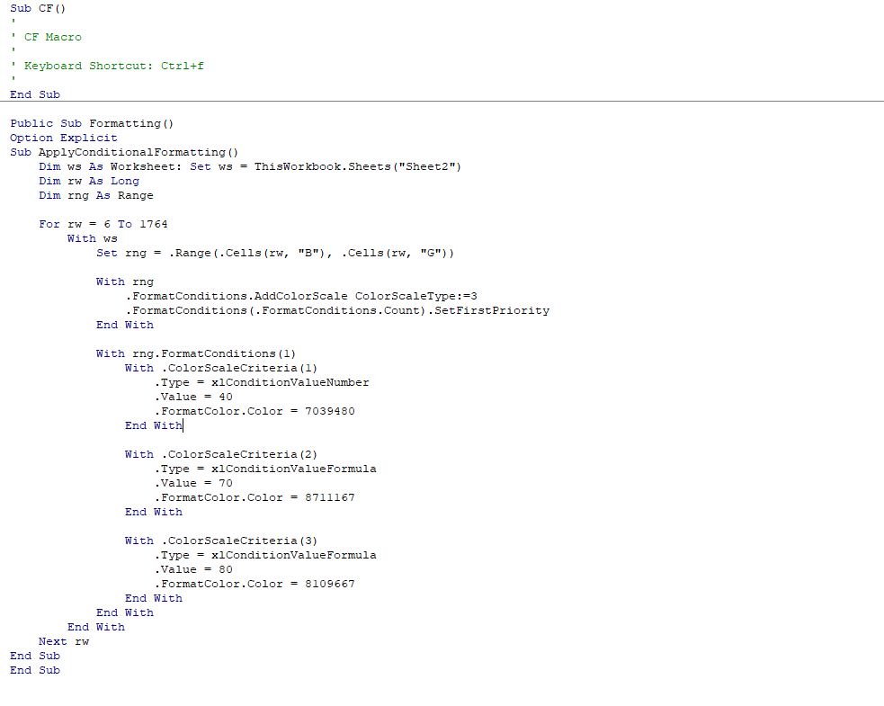
This code in theory would just be a blanket format of all of the data in columns B-G, however I hoped that if it was able to automate the process in general it would be a start. So I changed the text to fit my needs (essentially the same macro) and changed the formatting rules to format based on numbers:

When I try to run the program nothing happens- and I am wondering if a piece of the code is incorrect. Additionally, what code would be required to format every three rows (with all three key figures present), and would this be the best way to automate this process in general?

Second question: 

Once this formatting is complete, I wish to copy the formatted colors in the six columns of the rows associated with Supplier Network DOH, and copy those colors without the rules or the values to the six Total Inventory cells below for each item. The purpose of this to be able to show with the use of conditional formatting Days on Hand risk- through color layered over the total inventory. I found a related article discussion: https://stackoverflow.com/questions/18548156/how-to-copy-the-conditional-formatting-without-copying-..., however copy and pasting just the color themselves did not work on my Windows 10 excel version. Is there a way to do this process as well?

Sorry for the long questions- but I would appreciate any help I can get.

[#2]

@adisera 

Here was the code- I didn't realize it came out weird in the text box.