Changing vlookup array based on a cell value

[plzsiga]

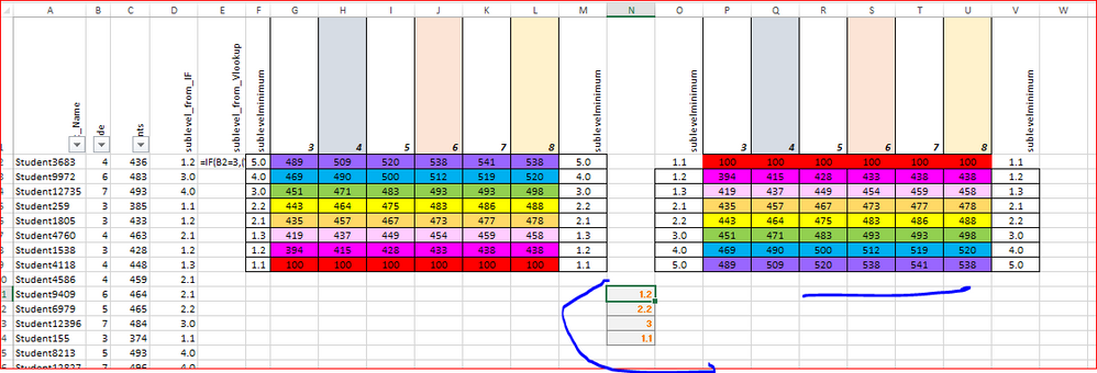
There are different classifications for scores based on a student's grade.  I can do multiple IF statements (see column D), but that requires filtering by grade and editing the formula several times.  Is there a way to do this with a Vlookup?

This does not work (see E2):

=IF(B2=3,(VLOOKUP(c2,$f$2:$g$9,2)),IF(B2=4,VLOOKUP(c2,$f$2:$h$9,2)),IF(B2=5,VLOOKUP(c2,$f$2:$l$9,2)),IF(B2=6,VLOOKUP(c2,$f$2:$j$9,2)),IF(B2=7,VLOOKUP(c2,$f$2:$k$9,2)),IF(B2=8,VLOOKUP(c2,$f$2:$l$9,2)))

[#2]

@plzsiga 

If it's possible to keep your sub level range in reverse order

the formula could be easier, like

=VLOOKUP($C2,INDEX($O$2:$U$2,$B2-1):$V$9,10-$B2)

If I understood your logic correctly.

[#3]

@plzsiga

Hi,

Please check out the below formula:

=INDEX($F$2:$F$9,
IF(ISNUMBER(MATCH(C2,INDEX($G$2:$L$9,,MATCH(B2,$G$1:$L$1,0)),0)),
MATCH(C2,INDEX($G$2:$L$9,,MATCH(B2,$G$1:$L$1,0)),0),
MATCH(C2,INDEX($G$2:$L$9,,MATCH(B2,$G$1:$L$1,0)),-1)+1))

Hope that helps

[#4]

Thank you! Than worked perfectly, too, and the 'reversed' order was the original from the source.

[#5]

Hatham, Thank you! It worked! It also was more accurate than my original code submitted. I guess I'm going to have to explore the INDEX and MATCH functions.