Alternated coloured columns - in pairs

[Deleted]

I've got a spreadsheet where all columns (apart from headings in col A) are in pairs. I would like all pairs of columns to be shaded in simply alternate colours. 

So Cols B&C would be very light blue, D&E very light grey, F&G very light blue etc.

I've found plenty of google hits explaining how to do this for single columns, but I've not been able to find a solution for pairs of columns.

Incidentally, I'd still like all cell borders to be visible (default colour being fine).

Any suggestions would be welcome.

Thanks

[#2]

I've just read that this should be in Answers.com. Very confusing Microsoft for us non regular visitors. I'll post it there. 

[#3]

I advise you to simply select the columns starting with row 2 and apply fill the pertinent fill color. If you prefer conditional formatting, which I personally dislike for being volatile and thus slow down calculations, select the pertinent range and apply these conditional formatting rules:
For very light gray: =(AND((MOD(COLUMN(),4)=0),(MOD(COLUMN((),4,)=1))
For very light blue: =(AND(ISEVEN(COLUMN()),ISODD(COLUMN()))
Ensure that you check the box for Stop if true for rule 1.
The choice is yours.

[#4]

@Deleted 

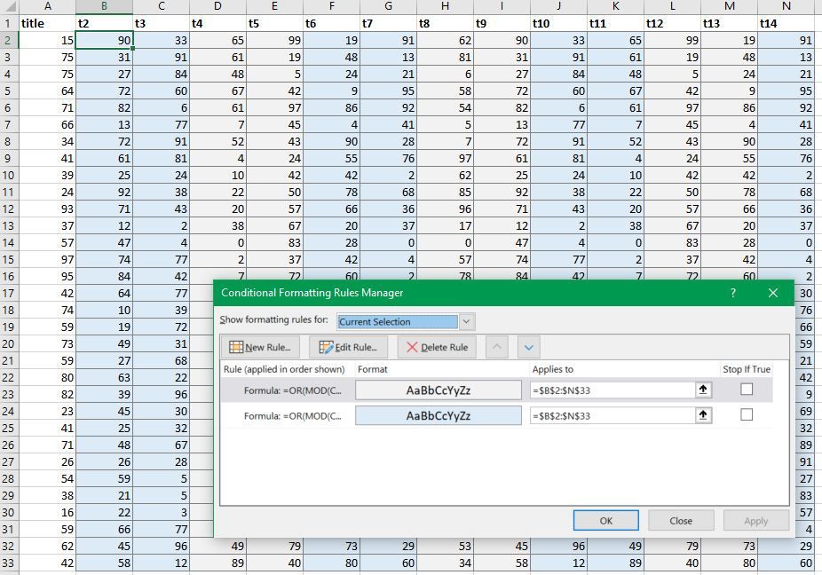
you can use conditional formatting.

the formulas for the conditional formatting showing on the picture are:

=OR(MOD(COLUMN(B2)-COLUMN($B2),4)=2,MOD(COLUMN(B2)-COLUMN($B2),4)=3)

and

=OR(MOD(COLUMN(B2)-COLUMN($B2),4)=0,MOD(COLUMN(B2)-COLUMN($B2),4)=1)

When indicating the format to apply with each rule choose a color for the interior of the cell and a color for the border.