Advanced Conditional Formatting?

[Fyse Jamali]

Hello,

I am looking to create a table with a list of individuals who have completed a specific training and have received a certificate for it. Let's say for example it is CPR Training.

I visualize the "indiviudal's name", the "type of training" and the "date" the training was completed / certificate was received.

What I would like to do is format the "date" cells to change colour. For example, if the CPR training certificate for a specific individual was received on April 17th, 2018 and the training is valid for 2 years (before they need to redo it) (i.e. April 17th, 2020) then I would like the colour to change of the "date" cell to yellow 3 months prior to the expiry date (i.e. starting January 17th, 2020) up until the expiry date at which point it would change to red (indicating that the training certificate is no longer valid and the individual must complete the training again)

I hope this makes sense :)

Thanks for the help!

[#2]

Hi Fyse,

You may apply conditional formatting rule like

=(EDATE(<date>,24)>=EDATE(TODAY(),-3))*(EDATE(<date>,24)<=TODAY())

for yellow color and

=(EDATE(<date>,24)>=TODAY())

for the red one

[#3]

Hi Sergei,

Thanks for the reply, I really appreciate it. However, I am still unsure of how to continue with this.

Could you see the attached example file and help me out?

Much apprecaited,

Fyse

[#4 · Accepted solution]

Hi Fyse,

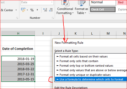
Select your dates, in ribbon Conditional formatting, New rule, Use formula...

Add formula

=(EDATE($H5,24)>=TODAY())*(EDATE($H5,21)<=TODAY())

and apply yellow format

Ok and apply

Repeat Conditional formatting -> Manage rule, New rule, etc, but with formula

=(TODAY()>=EDATE($H5,24))

Result is like this

and attached.

Sorry, I was wrong with previous variant of formulas, corrected.

[#5]

Hi Sergei,

For the longest time, I couldn't figure out why I was not getting any yellow boxes. I realized in my dates, I did not leave an example for a yellow cell. But, you adjusted the date to show it. Everything works perfectly! Thank you so much for this, I appreciate it!

Fyse

[#6]

You are welcome