Excel - Line Graph adds data series as graph title, ignores one data series for no reason.

[Chris Drinkall]

Please see attached file (Is Excel 2010 format, no I cant update it's a works computer).

I have been tasked with measuring the latency as we are having connectivity issues. Part of that requires a graph to be made visualising the latency data. According to all help files this should be so easy. But it's not.

What I need is someone to tell me what needs doing to make the graph as described below. I will be providing daily reports so will be using formulas to strip the latency from columns E and F and display the results in columns C and D as in the spreadsheet.

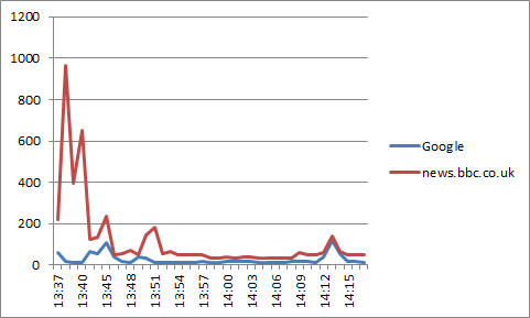
The graph simply needs to have column B be the horizontal axis, and plot lines using the numerical data on rows C and D. This shouldn't be rocket science. I am guessing it's freaking out due to some column not being formatted correctly. Column C and D MUST contain formulas to make the process quick.

Please confirm the steps to take to make this work. I am ashamed to admit excel has let me down here, colum B is formatted to "hh:mm", and C+D are numerical already.

[#2]

Hi Chris,

1) Convert C and D to numbers, they are text now

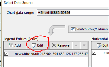
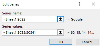
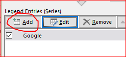
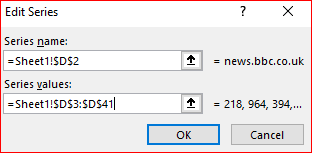
2) Right click on graph, change series on C and and add another series from D

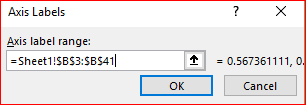
3) Edit here horizontal axis and select B

Please see attached

[#3]

Hi I don't know what you mean in step 2 "change series to C" there is no "change series" option in the right click menu. You have to explain every step in full detail. I've never made a graph in 2010 and at this rate never will. Imagine explaining it to your grandad!

[#4]

Okay,

Step 1

Step 2

when

when

with

after that

and

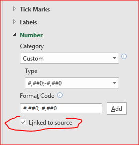
Double click horizontal axis now to format and link to source

Now you may do some cosmetic - stay on chart, Chart tools section will appear in ribbon, at very left under Add chart elements you may add/change title, labels, etc.

[#5]

Thanks for trying but it's still not there. I don't know what "format" options I should use (in the last step). The verticle side of the chart is showing 0.00 at bottom to 1.00 at the top.

Even if I click on this and change the maximum to 3000 (so all the numbers are within that range so should be drawn), no lines are drawn.

[#6 · Accepted solution]

Chris, step by step.

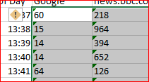
Most probably vertical axis is from 0 to 1 since you didn't convert values in columns C and D from text to numbers. To check, in any empty cell you may enter

=ISNUMBER(C3)

if FALSE you have text.

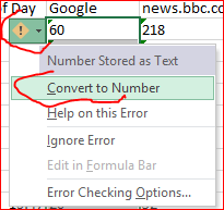
It shall be green sign at top left corner of each of such cell

If so the easiest way to convert is to select all such cells in C and D, you will see the icon on the top left of selection

Focus the mouse on it and from drop-down menu select Convert to numbers

Does it work?

[#7]

Format axis on Step 3 is for the horizontal axis to show your time as in table, in time hh:mm format, not as numbers.

[#8]

It would appear that using format cells > number does not work!? I am non the wiser as to why that wasn't working or why in the "home" ribbon it was showing those columns as numbers when they were not. But using isnumber() is was able to diagnose the problem. This did fix it.

I was also able to quickly find the solution to my further query, for those interested, as where column C+D are in the example already "numbers" they are formulas in the proper spreadsheet. Using value() on any output will convert it to a number.

[#9]

Chris,

1) In most cases if your values are at the left side of the cell they are text, numbers are aligned to the right site. As far as you din't apply any alignment formatting.

2) Green sign in the cell is also a good sign what you may have wrong format

3) Just format the cell from text to number won't affect values already entered. You shall re-edit your cells to apply new format. As an example you may press F2 on any of such cells and Enter - it'll be converted to number

4) I'm not sure about your formulas, perhaps that's more easy way to return numbers. But yes, VALUE() shall work.